From Outliers to Process Anomalies: Predictive SPC. Part 3

Predictive SPC. Part 3

Statistical Process Control (SPC) is a well described framework used to identify weak points in any process and predict the probability of failure in it.  The distribution parameters of process metrics have been translated into process capability, which evolved in the 1990s into the Six Sigma methodology in a number of incarnations. However, all techniques derived for SPC have two important weaknesses: they assume that the process metric is in a steady state and they assume that the process metric is normally distributed, or can be converted to a normal distribution.  The concepts and ideas outlined here make it possible to overcome these two shortcomings. This method has been developed and validated in collaboration with Josep Ferrandiz.   This is the third post in the series on Predictive SPC.

Definitions are here.

In Part 1, we covered the Axioms and Assumptions (A&As) of SPC, explained why they are wrong, but useful.  In Part 2, we talked about the key concepts and ideas of SPC,  and now we move on to how the key SPC concepts and ideas will change if we consider non-stationary processes.

Non-stationary processes

For stationary processes, we measure defects per million opportunities, or cases when the process is outside the specification limits.  If we have established control limits, then violations of these are considered defects.

But what if we have a runaway process that has not yet hit the specification (or even control) limit, like in Figure 2?

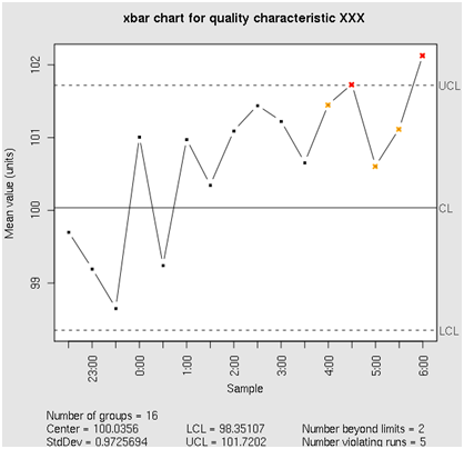
Figure 2: A runaway process

In this case, can we notice that the process is getting out of control before it hits the specification limit?  If we can, then do we need to “fix” it?

The answer to the first question is yes, we can notice the trend in the process metric.  A number of methods used in Time Series Analysis (TSA) will work here, most common being the correlation analysis.  In this case, we check if there is a statistically significant correlation between the timestamp (“Sample” in Figure 2) and the process metric.  The standard Pearson’s correlation will do it for most cases, but it will miss nonlinear monotonic correlations, which are just as important.   It is better to use Spearman’s correlation test instead.

The answer to the second question is not as obvious.   A statistically significant trend in the time series means that there is an external process forcing the metric to change, and the question becomes, do we need to worry about it, or has it always been like that?  In other words, we need to determine whether it is “normal” behavior of the process metric.

There is infinitely more to time series analysis than we have outlined in these couple of paragraphs.  For more details, please see, e.g., [4].

Trend in an Independent Variable: Time-Series Approach

The easiest way to benchmark a process is to look back and to compare the latest data against the old.  If the metric has always been behaving like that, it means that “it is what it is”, the process is experiencing organic growth, and nothing has really changed.

Correlation to time

The idea is to compare the correlation coefficients to time for the baseline and for the recent data.  If the correlation has not changed, it is “business as usual”.  If it has, then we probably have what Box and Luceno [2] call “attributable cause” behind the change in data behavior.   

To do such analysis, it should be possible to perform the T-test on the correlation coefficients for the baseline period and for the latest period of time.  The correlation coefficients (Pearson or Spearman), however, do not support such comparison: they are not normally distributed; therefore, the basic assumption of the T-test will not be true.  Fortunately, Fisher transform allows us to perform a T- (or Z-) test on the transformed value of the correlation coefficient.

Time-Series Analysis: Regression to time; EWMA; Holt-Winters; ARIMA

Exponentially-weighted moving average, or EWMA (with the Holt-Winters modification to account for the trend and seasonality), predictive filtering is a solid way to benchmark the data: indeed, if we assume that we have a Markov process (the next data point value only depends on the one immediately prior to it), then it does not matter whether the baseline data set is longer than the latest data set, and we can just compare the Holt-Winters predictions.  Alternatively, the ARIMA forecasting technique can be utilized.  

A definite advantage of the Holt-Winters and ARIMA approach is in that it allows for optimization of the parameters defining how fast the importance of the data point decays as the time goes by.  This can be described, in the Holt-Winters case,  as a nonlinear-programming (NP) simplex optimization problem.

In-depth discussion of the techniques and their advantages and drawbacks is outside the scope of this paper.  For more details, a number of good text can be recommended, most notably [2], [4], and [5].  Each of these methods can produce a prediction of the process metric with some degree of uncertainty.  This degree of uncertainty is quantified by the Predictive Interval, or PI, of the forecast.

If the latest data has come outside the Predictive Interval (PI) of what the model said based on the baseline data, then we have a problem.  If it is still within the PI, we are ok, and the organic growth is “as expected”.

Selection of the Best Approach to Benchmarking for Time Series Analysis (TSA)

A number of factors play a role in the selection of the best technique, or combination thereof, for SPC through benchmarking.  Ultimately, it all depends on the data behavior, and as is usually the case, there is no one-size-fits-all solution.   

Whatever the chosen method for selecting the best approach, it all boils down to what is nowadays called machine learning, but really is an automated trial-and-error (T&E) methodology on steroids, since lately massive parallelization has allowed analysts to run multiple models in parallel on the same data sets, selecting the best fitted model when finished, thus reducing greatly the time it takes to compute the forecast.

In addition, the recognition being finally granted lately to the Bayesian methodology, and the development of the “thermodynamics of information” have in the last 15 years made it possible to fit models so as to avoid overfitting and to make likelihood methods, as well as survival modeling, really attractive to the analyst.  

Adaptive Alerting (the credit for this section belongs to Dr. Josep Ferrandiz; his blog is here)

Adaptive alerting can be viewed as an application of time-series analysis on steroids: the goal here is to find, at each data point, the new threshold and to verify whether or not the new data point is outside that threshold.  In other words, adaptive alerting can be formulated as the problem of detecting statistically significant events as they are happening.  In a sense, it means going from an arbitrary physical threshold to a statistically sound percentile (probability) threshold.

Two approaches to Adaptive Alerting

Entropy-based event detection

There are several entropy-based methods of event detection, from traditional Shannon’s entropy-based methods (e.g., the max-likelihood group of methods), to methods based on Second Law of Thermodynamics.  

Most notable among the Shannon’s entropy-based methods include max-likelihood methods, among which the most practical are methods based on Akaike Information Criterion (AIC) and Bayesian Information Criterion (BIC).  These methods have found wide application in a number  of applications, from multidimensional and polynomial regression (keeping the number of variables, or number of degrees of the polynomial, low) to multidimensional clustering.

Methods based on the Second Law of Thermodynamics take advantage of the notion that in a closed system entropy does not decrease.  This offers a very efficient way to detect events: entropy going down means the system is not closed anymore, meaning that an external event has changed the system’s behavior.

Residuals-based event detection

Here we compute the best-fitted model (regression or TSA - EWMA and ARIMA) and look at the residuals. An outlier in residuals is an event, and its significance is what determines whether we should alert on it or not.

The standard methodology of hypothesis testing works very well in this case, as it answers the question, “What is the probability that the variable value (or the model residual) will be equal to the one measured if we assume a given distribution of the data?”  The given distribution is either the actual distribution of the historical data (or model residuals) or a fitted standard distribution.

Other methods (e.g. [6]) offer innovative ways to use residuals for change-point detection in multidimensional data, where there is a correlation between the two data sets.  Time-Series Analysis (TSA) can be interpreted as a special case of multidimensional data and therefore the methods outlined in [6], [8], and a whole host of other publications, can be - and has been - successfully applied to TSA as well.

Stay Tuned for Part 4: Bringing It All Together!

From Outliers to Process Anomalies: Predictive SPC. Part 2

Predictive SPC. Part 2

Statistical Process Control (SPC) is a well described framework used to identify weak points in any process and predict the probability of failure in it.  The distribution parameters of process metrics have been translated into process capability, which evolved in the 1990s into the Six Sigma methodology in a number of incarnations. However, all techniques derived for SPC have two important weaknesses: they assume that the process metric is in a steady state and they assume that the process metric is normally distributed, or can be converted to a normal distribution.  The concepts and ideas outlined here make it possible to overcome these two shortcomings. This method has been developed and validated in collaboration with Josep Ferrandiz.  This is the second post in the series on Predictive SPC.

Definitions are here.

In Part 1, we covered the Axioms and Assumptions (A&As) of SPC, explained why they are wrong, but useful, and now we move on to the Anatomy of SPC Charts and some of the key SPC concepts and ideas.

Anatomy of an SPC Chart

A lot has been said in the literature and blogosphere about SPC charts; some have taken it to new levels, like Igor Trubin, whose Statistical Exception Detection System (SEDS) is described in his blog.  SEDS is an advanced “classic” SPC engine that is scalable enough to be used as an enterprise-level system.  (We met at the CMG’06 Conference where I was presenting my first CMG paper - A priori Evaluation of Data and Selection of Forecasting Model, which we had written in collaboration with Michael Perka who has been my guide into the world of IT for many years now - and have been discussing Capacity Management, Mathematics, and Philosophy every time we get together, writing up ideas on napkins and posing questions that inspire new publications.)  

This post describes the SPC chart, introduces some SPC rules of thumb, and discusses “classic” Statistical Process Control.  For more details, I highly recommend the book by the one of the greatest applied statisticians of our time, George Box, [Box, G.E.P, Luceno, A. (Eds.) (1997) Statistical Control by Monitoring and Feedback Adjustment; Wiley Series in Probability and Statistics; Copyright 1997, John Wiley and Sons, Inc.; ISBN 0-471-19046-2]

Figure 1 demonstrates a typical SPC chart of a single process that is within the specifications, but out of control.

Figure 1:  A process within specifications (UCL LSL ), but out of control.

If it is a time series (all data points are measured at constant time intervals), then all methods used in time series analysis are applicable to the process described by a chart like in Figure 1.

In this particular example, we see that the process is stationary (there is no trend in the data), but there are two problems: the mean (the magenta dash line) is off target (the blue solid line in the middle), and there is an outlier (data points marked with a red triangle).  In addition, the later half of the run points is on one side of the target, while in the earlier half of the run most of the measurements were on the other side.

We could use a number of standard outlier detection techniques here to identify such data points (you can find some of them here or here), and we could use the standard T-test to check that the mean of the data is below the target.  For more details on classic SPC techniques, see the Box & Luceno book..

Making things more interesting

If we have a number of similar processes (e.g., widgets coming from a number of machines, or CPU utilization in a data center across servers, or SAT tests results from one school district) characterized by time series similar to that in Figure 1, we should be able to bundle them up, introducing not only distribution in time, but also distribution across the bundle.

In this case, the variance that goes into the T-test (as standard deviation, or square root of the variance) and into the ANOVA (as variance) becomes

The number of data points becomes:

And the data points that we saw in Figure 1 as outliers may very well turn out to be regular data points.

How do we measure the quality?

For measurement of the process quality, two standard parameters have evolved and become the lingua franca of SPC:

In other words, if the data follow normal distribution, we want  to be better than a certain “critical” number (the higher the better), and we want to be better than a certain “critical” number (the higher the better).

As commonly accepted rules of thumb, it is customary to use Z = 6  as a lofty goal and Cpk = 1.33 as another lofty goal.

The Z Score:

The reasoning behind the critical number for the Z score is as follows:  if we have Z = 6.0, it means that we have zero defects – an impossible scenario.  For most industries, this requirement can be relaxed:  Z = 4.5 translates into a defect rate of 3.4 / 1 million, or 3.4 Defects Per Million Opportunities (DPMO).  

Parenthetically, The Holy Grail of Six Sigma methodology, Z = 6.0 goal is for short-term slices (samples) of the process; the samples are assumed to be distributed so that their range accounts for 1.5 Z-scores (for details, see the F-test assumptions).  That means that the short-term Z = 6.0 is really long-term Z = 4.5

A paradox:

If we look at civil aviation, 3.4 DPMO translates into 1 aircraft failure in midflight every 3.3 days.  Indeed, according to http://1lawflying.wordpress.com/2008/11/04/how-many-flights-per-day-do-air-traffic-controllers-handle-in-the-united-states/, as of November, 2008, every day there were 87,000 simultaneous flights in the skies over the United States. That means that a million flights (opportunities to fail) is accumulated in 1,000,000 / 87,000 = 11.5 days, and allowing 3.4 of these to fail means that on average every 11.5/3.4 = 3.38 days a flight is allowed to fail.  Nobody would want to be on that flight; so the critical Z score for civil aviation should be higher than 4.5.

The solution to this paradox is really quite simple if we consider the distribution of failures. Failure arrivals are always a process skewed to the left - typically, Poisson (although in some models Pareto, Weibull, and other heavy-tailed distributions are used); in other words, failure interarrival times (Times Between Failures – a measure used in reliability analysis) can typically be assumed to be exponentially distributed.  Aircraft injection into the airspace (takeoff or flying into its scope) and removal from it (landing or flying out of its scope) are also heavy-tailed processes.

A combination of these distributions will not produce a normal distribution under any circumstances. Therefore, the Z score, being devised as a measure of quality for a normally-distributed process, is not a good measure of the quality (and safety) of operation of the National Airspace.  This is another example of not allowing the CLT to mislead us.

The Process Capability:

Unlike the Z score, the Process Capability measures how far the process is from the specification limits.  It does not take into account how close to the target the process metric is, but it takes account of the fact that specification limits can be asymmetrical.  The 1.33 lowest limit is somewhat arbitrary: we want to leave a padding of 1/3 of the 3-standard-deviation range before we hit the upper or lower specification limit, whichever is closer (USL or LSL, respectively).  Hence

Cpk_min = 1.33 = 4 / 3 (5)

We have covered the anatomy of an SPC chart. Some of the concepts appear arbitrary (and are arbitrary), but are adjustable based on "what makes sense for the business". We'll talk more about business metrics in later posts in this series.

This concludes the section on Anatomy of an SPC Chart.  Stay tuned for Trended Time Series and SPC.

From Outliers to Process Anomalies: Predictive SPC. Part 1

Predictive SPC. Part 1

Statistical Process Control (SPC) is a well described framework used to identify weak points in any process and predict the probability of failure in it.  The distribution parameters of process metrics have been translated into process capability, which evolved in the 1990s into the Six Sigma methodology in a number of incarnations. However, all techniques derived for SPC have two important weaknesses: they assume that the process metric is in a steady state and they assume that the process metric is normally distributed, or can be converted to a normal distribution.  The concepts and ideas outlined here make it possible to overcome these two shortcomings. This method has been developed and validated in collaboration with Josep Ferrandiz.   This post starts a series on Predictive SPC.

Definitions are here

Part 1

State of the Art Today: Axioms and Assumptions

There are a number of excellent references to SPC in the literature and in the cyberspace, from George Box's classic books to a variety of Six Sigma web sites, including www.isixsigma.com.

Any reasonable cost-benefit analysis of using SPC says in no uncertain terms that when done right, it pays to keep the mean of the process on the target, and the control limits within the specification limits.  

Six Sigma is merely a goal that, according to its champions, every organization that cares about the quality of its products should pursue. This goal states that the variance of the processes should be such that there will be six standard deviations between the process target and either one of the specification limits.  That translates into 99.9997 percent of the product being within the specification limits, meaning that no more than 3 in a million units will be defective.

Extension of this statement brings us to an important concept.  If each unit of product is one opportunity for a defect, then with six standard deviations, we are guaranteed to have 3 defects per million opportunities, or 3 DPMO.  But if each unit represents multiple opportunities for a unit to be considered defective, then the DPMO rating will change.  

For example, if we are measuring the three dimensions of a box, and each of them has the same specification limits, then if we are trying to fit six standard deviations into the specification limits on each, we are talking about 3 defects per 3 million opportunities (one for each dimension), or 1 DPMO: the unit is defective if either one of the dimensions is off.  In other words, when we judge the defectiveness of an item by any one of many dimensions, we can relax the specification on the number of standard deviations, going, e.g., from 6 Sigma to 3.

Specification Limits and Target

Watch out:  Axioms and Assumptions (A&As)!

The goal of process control is to ensure that the process metric distribution stays within specifications.

Nonparametric analysis is usually computationally complex.  For this and other (mostly historical) reasons, the rivalry between Fisherian vs. Bayesian statistics having been a large part of this,  the primary methodology for SPC has evolved along the lines of the simplifying assumption of normal distribution, characterized by only two parameters,  mean and standard deviation.  

It is a convenient simplification that works for most cases, especially considering that many skewed distributions can be made normal by applying the Box-Cox and other standard transformations, and random sampling ensures the Central Limit Theorem works on the analysts’ side, driving the distribution of the means of the samples to normal.

This seemingly innocuous abstraction is very powerful, as it has made it possible to break down the absolute majority of SPC problems into three categories:

1.       Are we concerned about being off target?

2.       Are we concerned about being outside the specification limits?

3.       Are we concerned about both?

Answers to these questions are critical, because different statistical techniques have been developed for evaluating the processes, and care must be taken to use the right methods for each.

But there always is a fourth question:

4.       Are we concerned about something else?

More on A&As

SPC is resting on a solid theoretical foundation, and any theory rests on some basic assumptions.  They may be implicit, but they are nevertheless always present.  Since the goal of SPC is to implement stochastic control of variables that have a significant random component, we have to be aware of the assumptions implicit in the standard statistical tests.  

The main assumption is that the underlying distribution is normal (Gaussian).  If that is not true, then generally speaking, the T-test and the F-test will not work.

There are ways to make a distribution appear normal; there is the often abused Central Limit Theorem; however, it is important to remember that even if the Box-Cox transformation has been successfully applied, it does not change the fact that the underlying data are not Gaussian, and the symmetrical bell curve does not describe such data (more on that, e.g., here and here).

From the practical standpoint, it means that we cannot generalize the methods derived for the "classic" SPC, and that before we draw any conclusions about the data behavior, we have to always check the distribution for normality.

Parenthetically, even normality is not a guarantee of success: the samples have to be random and independent, and when it comes to sampling a time series, we run into the bigger issues of sample interarrival time distribution, distribution of sample durations, etc.

If we find (with or without the transformation) that the distribution is indeed normal, we can claim victory, because it means that the simple statistical tests derived by the classics will work, and they are what modern SPC is using.

A few more words about Central Limit Theorem and distributions

The Central Limit Theorem (CLT) states that no matter what the distribution is of the population, random samples of sufficient size taken from this distribution will have their means appear normally distributed if the number of samples is "big enough".  It does not say that, thanks to CLT, “big data” will assuredly have a normal distribution of the data.  Nor does it say that we do not need to worry about the actual shape of the population’s distribution.  Ultimately, it all boils down to being able to detect data behavior on the distribution tails, and this is where the skew and the kurtosis (flatness) of the distribution matters.

What CLT does say, however, is that if we use the means of a sufficiently high number of sufficiently random samples from a data population, we will certainly deceive ourselves into thinking that the population’s distribution is normal.

Example1:

The Poisson distribution is known to describe a wide class of processes where we measure frequency of events. For more details, see [1].  What it means in practice is that the interarrival time of events described by Poisson distribution is distributed exponentially (we will not go through the details of mathematical proof of this statement here; any textbook on statistics will have it).  

This is the basis of, e.g., Erlang’s models used in traffic analysis.  (Erlang’s models connect the offered traffic, the number of parallel lines to serve the traffic, and the blocking probability. Initially created for use in telephony, they have by now entered a wide variety of applications from highway design to IT capacity planning.  For more details, see [Josep Ferrandiz, Alex Gilgur. Level of Service Based Capacity Planning.  - 38th International Conference of the Computer Measurement Group (CMG’12), Las Vegas, NV, December 2012].)

However, if we have hundreds of transactions arriving and processed within an hour, and the only metrics we have are the hourly average arrivals for the hour and the hourly average processing times, we will be deceived into thinking that we cannot apply Erlang’s models - which is not necessarily true.  For more details, see, e.g.,  [Josep Ferrandiz, Alex Gilgur. (2012) Level of Service Based Capacity Planning. – published at the 38th International Computer Measurement Group (CMG12) Conference, December 2012, Las Vegas, NV.]

Finally (about A-and-As)

It is a useful deception, and we will use it to describe the SPC concepts.  Later in this series, though, we will see if we can take off the blinds and use the same principles with distributions that we know cannot be normal (or know nothing about).

Stay tuned! Next post will outline the Anatomy of an SPC Chart