Discovering Patterns in Irregular Behavior: Part III

ABSTRACT

Mathematical description of irregular behavior is the holy grail of statistical analysis, akin to a game of croquet that Alice reluctantly played with the Queen of Hearts.  (If you have not read or watched Lewis Carroll’s classic, please refer to a brief description of the game here.)  A lot of uncertainty and ambiguity, just like in the world of data.  In this section, we will discuss one very specific pattern that is critically important in a wide variety of fields, from cardiology to speech recognition, namely seasonality detection.  

A Few Words about Seasonality Definitions

First of all, regardless of what Wikipedia says on the page related to Forecasting, seasonality only in some cases has something to do with the four seasons.  Or rather, seasonality that is related to the four seasons is only one very special case of seasonality.  Wikipedia gives the “right” definition of it on the Seasonality page:  

“When there are patterns that repeat over known, fixed periods of time[1] within the data set it is considered to be seasonality,seasonal variation, periodic variation, or periodic fluctuations. This variation can be either regular or semi-regular.”

This is the seasonality that we are going to discuss here.

Seasonality Detection Methods

The most basic method of seasonality detection is to ask the SME (subject-matter expert).

Most SMEs will tell you that their data have a diurnal (a fancy word for “daily”), a weekly, or an annual pattern.  But few will tell you that they know what’s going on when the data don’t support their claim.

At this point, we might as well abandon hope to get any useful information from the human SMEs and dive into what the exciting world of machine learning, which in reality is nothing but no-holds-barred advanced statistics, applied, in the seasonality detection use case, to time series.

What is a Time Series?

Time Series is, according to Wikipedia’s article, “a sequence of data points, typically consisting of successive measurements made over a time interval”.  NIST is more precise in its definition:  “An ordered sequence of values of a variable at equally spaced time intervals”.  This definition is the only invariant in time-series analysis.  Colloquially, sometimes the word “ordered” is replaced with  “time-ordered”.  

Seasonality Detection in Time Series

Why?

The most obvious answer to the "why" question is clear from the main use case of Time Series Analysis, - forecasting.  Indeed, predicting future behavior of a seasonal time series without accounting for seasonality is akin to driving a small square peg into a big round hole: it fits, but the precision of such model will be poor.

Other use cases include speech recognition, anomaly detection, supply chain management, and stability analysis.

How?

The standard seasonality detection methods, like Fourier analysis, domain expertise, autocorrelation function, etc. work fairly well in most scenarios.  

However,

• Domain experts are primarily humans
• Autocorrelation -based seasonality detection involves thresholding, which is only one step better than domain expertise-based seasonality analysis
• Fourier analysis often leads to models that overfit the data

This means that what we are left with is two extremes - too generalized (human) or too specific (Fourier analysis).

An illustration

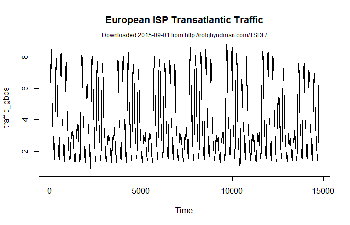
Figure 1: Transatlantic traffic data from a European ISP.  Data cover June-July of 2005.  

Data downloaded from this URL on 2015-09-01

The data are flat enough that we can use this data set to illustrate the concepts we are about to introduce here.  To deal with fewer data points, we will go to hourly medians:

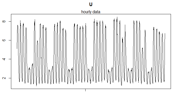
Figure 1a: hourly medians

While it seems fairly obvious visually that there is a daily and a weekly pattern in the data, standard methods will not be very useful.  For instance, the AutoCorrelation Function (ACF) returns pretty much the entire spectrum as frequencies:

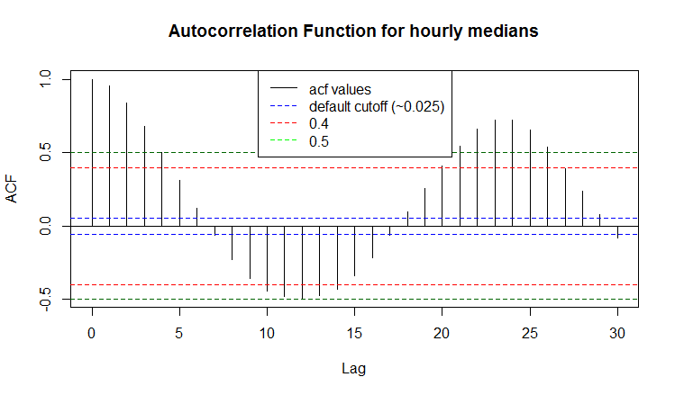
Figure 1b: ACF

Bars whose absolute values are outside the dotted envelope traditionally represent the seasonality.While there is a reason behind the default value of 0.025 (the reason being in Fisherian statistics: if ACF is outside the 5% envelope, we cannot say with 95% confidence that the data are not seasonal); it is clear that with complex seasonal patterns like shown in Figure 1, it is not very meaningful.  Expanding the confidence envelope even to 50%, does not contribute much information to our knowledge about these seasonalities.  

Looking at Figure 1, we also notice that the upper and the lower parts of the data follow very different patterns: the maxima follow a 2+5 pattern, while the minima follow a daily rhythm with a slight weekly rhythm.  It is understandable if we recall that these data correspond to traffic through a large Internet Service Provider (ISP) in a very busy time of a year - June/July.

Let’s follow through with the ROC idea and see where it brings us.

Figure 3: ROC time Series plot.  

Points following ROC change of sign are marked as red dots; all others are blank dots.

Figure 4.  Hour-to-Hour variability in traffic

In Figure 4(b), the points after which the sign of the first derivative changed from positive to negative correspond to the local maxima of the hourly median time series.  They are marked as blue filled dots. Points where second derivative changes sign are inflection points.  These are marked as boxes.

Let us look at the distribution of the time intervals between the sign-change points.

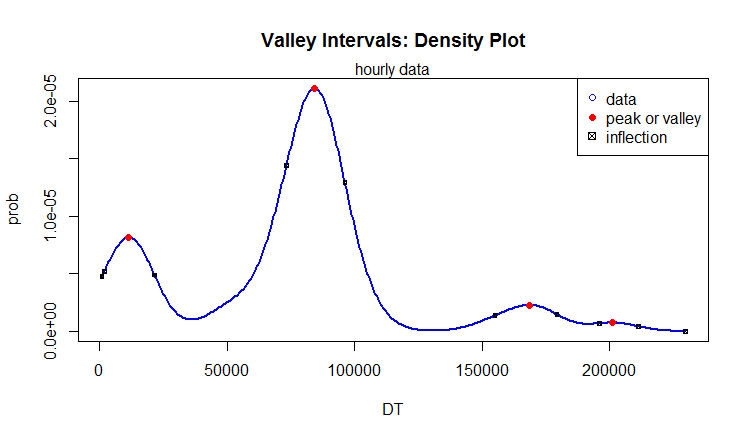
We see that the density plot, too, has multiple local maxima.

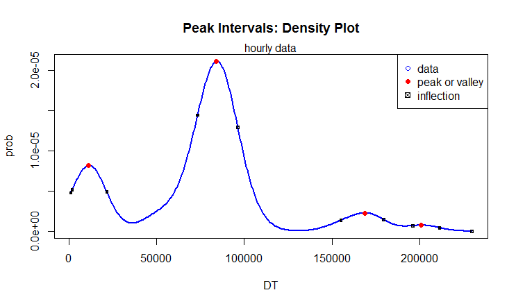
(a): Distribution of intervals between peaks (seconds)

(b): Distribution of intervals between valleys (seconds)

Figure 7: Density of time intervals between local maxima and minima of hourly traffic medians.

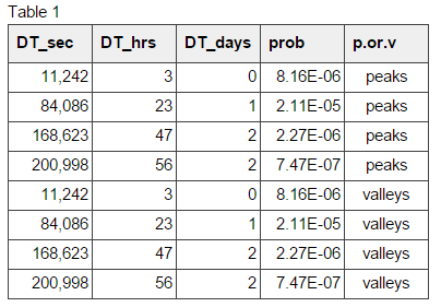
We see from Figure 7 (a & b) that peaks and valleys of the hourly traffic medians follow the same pattern.  Table 1 verifies this.  The peaks are observed at 3, 23, 47, and 56 hours, and so are the valleys.

Their complex interactions and interferences, not unlike the Wave Pendulum, produces the pattern we saw in Figure 1.

Conclusion
We have demonstrated a reliable method of detecting complex seasonal patterns in time series data. This method does not require Fourier decomposition, regression fitting, Neural Networks, or any other overkill techniques.  All that is needed is high-school Calculus, Probability and Statistics, fundamental understanding of Clustering, and a little common sense.

CMG2015 Performance and Capacity International Conference

The #CMG2015 conference was an overwhelming success.  I have not been able to find a paper that would not be interesting, and all presentations were engaging, enlightening, and deep.  Not only was it a breath of fresh air - it always is that! - but also it was a great opportunity to learn and to network with the world's best IT Performance and Capacity experts.

The level of academic rigor and practical expertise at CMG Conferences is huge and growing.  It is not a trade show, and it is not a purely academic event, but something unique, and I really hope that it will continue in this direction: this way, CMG will grow in numbers while upholding its reputation as the only organization of IT professionals where academic knowledge and technical expertise have united to form this unique alloy that has been attracting us to keep coming to CMG Conferences again and again.

Our paper, "Percentile-Based Approach to Forecasting Workload Growth",  has got a lot of good attention too, and I received the prestigious Mullen Award for presenting it!

Thank you, CMG!  I really hope to see you all in La Jolla at CMG2016!

"Percentile-Based Approach to Forecasting Workload Growth"

It is the title of our paper that has been accepted to the Performance and Capacity (CMG'15) International Conference that is taking place in San Antonio, first week of November.  If you were a Conference referee who let it happen, THANK YOU!!!

If you are going to the Conference, I am presenting the paper on Thursday, November 5, at 10:30 AM in Naylor (Session 525).  I'll be happy to see you there!

Discovering Patterns in Irregular Behavior: Part 2

Mathematical description of irregular behavior is the holy grail of statistical analysis, akin to a game of croquet that Alice reluctantly played with the Queen of Hearts.  (If you have not read or watched Lewis Carroll’s classic, please refer to a brief description of the game here.)  A lot of uncertainty and ambiguity, just like in the world of data.  Could Alice have won the game?   

About Previous Post

In the previous post, we set the scene and explored the history of the problem.  If you want to read about it from the sage who actually made the history of modern data science, you should get offline and read the book “An Accidental Statistician” by George Edward Pelham Box - the father of modern statistics.  Sadly, he passed away in 2013 at 93 years of age.  He was one of the titans of statistics responsible for design of experiments, statistical quality control, time-series analysis, evolutionary operation, useful transformations, and the return of Bayesian methods into the mainstream of Data Science.  The true impact of his work will be reverberating for many decades.

We also started a discussion of what Data Science really is, and explained briefly how the two new approaches were enabled by technology to become the two prongs of the never-ending attack on data: Monte-Carlo became the method of choice that eliminated the need for pigeonholing distributions, while Machine Learning became the tool that promised to eliminate the need for a human in the loop of data analysis, setting us free of the burden of mechanical crunching of data and giving us time to think.

Enter Random Events: the Biggest Paradox of Data Science

When it comes to random events, we tend to go long circuitous routes in order

to bring random events back into the fold of the Familiar. Paradoxes tend to scare us.  We are like Alice, sharp enough to see the differences between how we think the world works and what we see, but clueless what to do about these discrepancies.

What Would Bohr Do? We have a system whose behavior we think we know.  When we say “we know behavior of a system”, what we really mean is that we can predict its behavior at any moment in time with a satisfactory degree of certainty.  The system is predictable, self-consistent, “sane”.  We know the distributions of the data and can determine the tolerances that put us into given confidence intervals.   But then - blame Murphy’s Law, or Gȍdel’s Incompleteness Theorems, or any of a number of conspiracy theories - life throws us a curveball, and the system stops behaving the way we know it to behave.  We really run into a paradox: what we know about the system gets challenged, and our first feeling is crushed, because few of us can say calmly, like Niels Bohr: “How wonderful that we have met with a paradox. Now we have some hope of making progress” The paradox in modeling is similar to Bohr’s legacy: if we perfectly fit a model to its previous behavior, its predictive ability will be lower than if we build a model that does not fit 100% of the historical data.  The planetary model of the atom was not an oversimplification.  It was a generalization which, combined with evolutionary (some would call it Bayesian) approach to modeling, allows us to accurately model the world: “Essentially, all models are wrong, but some are useful”. What is in common between Alice playing strange croquet, our tea-making R&D team, and any data analytics expert? They all find themselves in a situation where observations do not fit their model.  This is not an unusual situation, and our three members of the tea-maker design team did what every rational person would do under the circumstances. Any change in initial conditions, environment, or observer's perception will have an effect on the parameters and even the structure of the model describing the scenario.

What do we do? Imagine that you asked a team of a physicist, a software engineer, and a mathematician to come up with an algorithm to make tea. There is little doubt that they will take no time completing the task: Pour water into a kettle Start heating the water in the kettle While it is coming to boiling (100oC / 212oF) , the operator has about 10 minutes to put the tea leaves (or a tea bag) into the cup(s). When the water has reached just a degree or two below 100°C (212°F), pour it into the above-mentioned cup(s). And then you preheat the tap water to 97°C (206°F) in an industrial boiler and ask each of them to individually validate the algorithm. The physicist will explain why it is impossible to have liquid water stored at its boiling point using nothing but household items, even after you show him that you have it stored. The software engineer worth his salt will most likely see the performance improvement you have just made possible by preheating the water and volunteer to rewrite the algorithm they all devised to make it more flexible while optimizing some of the code:  if you have multiple cups of tea to prepare, you could set them all up in parallel with the leaves/bags, and then if you can pour water into all cups concurrently... Finally, the mathematician will absentmindedly pour the hot water into the kettle, start heating the water in the kettle, put the teabag into the cup, using this time (while the water was being poured it cooled down somewhat), to contemplate the probability of such an event happening and what prior events could have led to it. He will be genuinely surprised that this time the water reached the boiling temperature so fast and will likely call his friend the physicist as the subject-matter expert and discuss it with him. Once they have agreed on a theory that the max-likelihood cause of this curious behavior was the significantly (both statistically and practically) higher initial temperature, they will invite the software engineer to a meeting, who will come immediately with three steaming cups of excellent tea made by applying his new algorithm to the preheated water. They will then proceed to ask him to redesign the program to account for the bizarre event of water initial temperature being higher than the expectation, and will show the equations that they will want him to use in his tea program. The next day, the abstract of a new publication authored by the three friends having to do with discovery of new properties of the kettle material will be on your desk.

With Data, Nothing is Ever Deterministic

As chaos theory suggests, deterministic behavior can lead to pseudo-random behavior, but the Second Law of Thermodynamics ensures that the opposite is not true.

In practice, any measured data value can be described as a sum or a product of two measures:

Additive Form

Multiplicative Form

Naturally, for the positive values of X_measured a simple log transformation can turn multiplicative form into additive:

and we get an additive form by reassigning:

If X_measured is zero or negative, the log function is not defined for such values, but we can “normalize” the variable (divide it by its range), bringing it into the (0, 1] range, where logarithm is defined.  Because such range normalization is done by dividing the value by the range, a more accurate form of Eq. (3) and Eq. (4) would be:

This works for the deterministic component of the measured value. However, the shape of the distribution of the stochastic component will change in a log transformation, leading to general smoothing out of the right tail of the distribution..

Deterministic Component

The deterministic component is what goes into the mathematical models when we attempt to understand how something works by writing equations to describe the physical behavior of the objects.  From Newton’s Second Law to general theory of relativity, we have been looking for, and finding, the equations that describe the world around us.  

Stochastic Component

However, when we ask ourselves how accurate our equations are, we run into validation issues.  The stochastic component can be confoundingly big, hiding the underlying laws of system behavior behind the guise of randomness (more about it, e.g., in an earlier post in this blog).

The stochastic component of the observed data point has two elements:

• Out-of-scope features - variables that are not accounted for in the model or in the data we have.
• Measurement error - an intrinsic property of the measurement system.  Error in estimating regression parameters also falls under this category.

These two are orthogonal (independent); therefore,

Because of the first element of the stochastic component, and the Incompleteness Theorems, data measured from a live process will never be purely deterministic.  Therefore, our prediction models can never be 100% accurate.

You Know What To Do

There are only two possible courses of action when it comes to randomness:

• embrace it and understand it
• embrace it and account for it in your models.

(To be continued)

Discovering Patterns in Irregular Behavior: Part 1

Discovering Patterns in Irregular Behavior: Part 1

Mathematical description of irregular behavior is the holy grail of statistical analysis, akin to a game of croquet that Alice reluctantly played with the Queen of Hearts, where the wickets (cards / soldiers) move from their posts to “fix” the game, the mallets (flamingos) look at the player just before the ball (hedgehog) is about to be hit, and the hedgehogs start rolling down the court before they are hit with the flamingo’s head.  (If you have not read or watched Lewis Carroll’s classic, please refer to a brief description of the game here.)  A lot of uncertainty and ambiguity, just like in the world of data.  And if you add the political aspect of the game (Alice is playing with a Queen after all, even if an imaginary one!), that makes it an excellent allegory of what happens in data science nowadays.  Could Alice have won the game? Should she have?   

Setting the Scene

Problem Statement

The rules of croquet are here. There are nine wickets and two stakes, placed in a certain pattern (topology), and each side needs to score fourteen wickets (going around the court and scoring one point per wicket).  Each time a wicket or stake is scored, the player gets one bonus shot for the ball that scored the wicket or stake.  The game is well structured, and the only uncertainty comes from the skills of the players and the strategy and tactics they are using.  

Mathematically speaking

We have a game G(N, p, b), with p players, b balls per player, and N wickets.  If blocking other player’s ball had been prohibited, then each player’s goal would be to maximize the number of wickets they score while keeping their “tank” of bonus shots sufficiently full, given the number and topology of the wickets and stakes:

Turn:P: max(W|B, Topo),

where P = player ID; H = number of wickets and stakes, B = number of bonus shots the player has, and Topo = the topology (layout) of the court (wickets, stakes, and balls).

Perhaps a better strategy would be to minimize the number of turns the player needs to finish the game given the number of bonus shots he/she has and the topology of the game:

P:min (NTunrs |B, Topo)

However, this is the trivial scenario, the non-interactive game.  In the interactive game, each player has more than one ball and is allowed to use either one to block the progress of the opponent to his/her goal by hitting their ball(s) with his / hers. The rules encourage the players to hit any opponent’s ball with theirs: while scoring a wicket is worth one bonus shot, hitting an opponent’s ball is worth two, improving their chances to finish the game before the opponent.  This changes the previous expression for the winning strategy to:

P:min (NTurns |B, Topo, Pr(other)) ,

where P = player ID, B = number of bonus shots the player has, Topo = topology of the game, and Pr(other) = probability distribution of actions by the other participants of the game (e.g., opponent).

Uncertainty

Without going into the details of game theory, suffice to say that the opponent’s behavior adds some uncertainty to the player’s strategy and tactics; however, this ambiguity is predictable given that each player knows what the end goal of the game is, and assuming the players keep track of each other’s bonus shots, they can predict what the opponent will do with a decent confidence and based on that build their own strategy and execution: it’s all about Pr(other).

“Curiouser and Curiouser”

These are the words immortalized by Alice when she remarked on the amount of ambiguity she is facing in Wonderland.  While grammatically incorrect, they do describe her point of view on what happened to her, especially at the Royal Game of Croquet.

The simple game with known rules changed ever so slightly - just adding another source of uncertainty, and Alice did not know what to expect anymore: her knowledge of Pr(other) was gone.  

Very quickly, she observed that the Queen’s mallet (flamingo) was solid and predictable , while the ‘wickets’ were moving to where the ball was rolling.  But whenever it was her turn to hit the ball, it did not work: her mallet -flamingo wanted to talk her out of it, ducked (pardon the pun!) just before it was hitting the ball, the ball would not budge, and the wickets were moving away from the ball.

Thomas Bayes meets Charles Lutwidge Dodgson

It is a well known secret that Lewis Carroll = Lutwidge Charles, and Dodgson = Dodo, the mysterious bird who, along with the Cheshire Cat, helps Alice figure things out in Wonderland.  What was in common between Bayes and Dodgson?

For starters, they were both clerics, the former a Presbyterian minister, while the latter an Anglican deacon.  They were both mathematicians specializing in logic, Bayes becoming known for the Theorem connecting unknown causes with observed effect and the whole methodology that is used today in statistics, while Dodgson, some 150 years later, became famous for popularizing complicated mathematical concepts, making them accessible even to a little child like Alice, even at the cost of becoming Lewis Carroll and Dodo (and maybe Cheshire Cat too? after all, he was born in the Cheshire county).

Bayes Theorem

The “classical” (traditional, frequentist, Fisherian) statistics, brilliantly formalized by Gauss, Gossett (known as the author of Student’s T-test), Fisher, Pearson, and so many others before and after them, and put to use by them for figuring out confidence intervals, correlations, required sample sizes, probability of making a mistake, and similarities between two distributions, - this side of statistics has been written and sealed into our brain since college.  Mathematical description of relationships between the explanatory variable(s) and dependent variable(s); statistical process control; mathematical forecasting and in general predictive analytics applied to continuous variables are all derived from the theoretical foundations created by these giants.  

They made beer produced in England survive the sea voyage to India; they made it possible hundredfold improvements in crop yields; they allowed scientists to figure out the laws of behavior of gases, liquids, and solids; predict the rates of chemical reactions; mathematically describe complex physical phenomena; extract signal from noise, and accomplish many other feats that would have been impossible without it.

At the same time, Bayesian approach, with its unassuming - pun intended here! -  approach to solving data-analytical problems, was the “Ugly Duckling” of the beautiful picture of the world, until it turned into a beautiful swan - not without the help of the statisticians who were more interested in solving the problems rather than admiring the edifice of Applied Mathematics.  Alan Turing, George Box, Diane Cox, and other brilliant mathematicians realized early enough that mathematics did not need to go into politics.  The gap between Frequentist and Bayesian statistics was bridged.

Data Science: Engineering? Machine Learning? Statistics?

In the 1920s, Goedel demonstrated mathematically that any non-trivial system of axioms is incomplete.  We compensate for this incompleteness by imposing confidence intervals and developing statistical methods to calculate these intervals for a given probability of making a mistake.

In the 1940s, scientists in the Los Alamos National Laboratory needed to model processes they had only a vague idea about.  They did have the mathematical models, but such models were not accounting for the incompleteness of our knowledge about the world they were peeking into.  The Monte-Carlo simulation was born.  

The idea was simple:  when we have the mathematical model, and the distributions of input variables are known, we can slice the distribution of the input variables by multiple percentiles and for all combinations of percentiles of inputs, apply the mathematical model.  The resulting output variables will have a distribution whose parameters can then very easily be evaluated.

The first electronic numerical calculating machine (ENIAC) had already been developed in the early 1940s.  Its computational speed made Monte-Carlo calculations feasible.  Nick Metropolis, Stanislaw Ulam, and John von Neumann were the founding fathers of modern Monte-Carlo method and the practical numerical approach to data analysis and modeling.

The amazing advances of the computing power, the computer engineering technology enabled an unprecedented fractalization and parallelization of mathematical tasks.  Models that only twenty years ago were rejected simply because they were too computationally intensive are beginning to take foothold and are leading to discovering new knowledge.  We are no longer confined to the Gaussian-distribution assumption about the data.  We are not even confined to any distribution assumption.

That, combined with Alan Turing’s definition of artificial intelligence, has enabled “machine learning” to step from the realms created by the minds of Isaac Asimov and Arthur Clarke into the world of philosophical and ethical discussions, psychology, and finally, Knowledge Discovery and Data Mining, or KDD.

For an idea to come into acceptance, it has to be demonstrated.  

Dr. Frankenstein chose the wrong time and the wrong place to demonstrate his creation to the world.

Starting in 2004, the DARPA Grand Challenge and other DARPA-sponsored competitions of artificial-intelligence devices have been conducted, highlighting different aspects of usability of such devices.  The common denominator among competing teams is their use of machine learning in near-real-time analysis of the situation in front of them and making decisions independently of their human handlers.

Hopefully, now the time and place is more fruitful than it was for Frankenstein.

(To be continued...)