Predictive SPC. Part 3
Statistical Process Control (SPC) is a well described framework used to identify weak points in any process and predict the probability of failure in it. The distribution parameters of process metrics have been translated into process capability, which evolved in the 1990s into the Six Sigma methodology in a number of incarnations. However, all techniques derived for SPC have two important weaknesses: they assume that the process metric is in a steady state and they assume that the process metric is normally distributed, or can be converted to a normal distribution. The concepts and ideas outlined here make it possible to overcome these two shortcomings. This method has been developed and validated in collaboration with Josep Ferrandiz. This is the third post in the series on Predictive SPC.
Definitions are here.
In Part 1, we covered the Axioms and Assumptions (A&As) of SPC, explained why they are wrong, but useful. In Part 2, we talked about the key concepts and ideas of SPC, and now we move on to how the key SPC concepts and ideas will change if we consider non-stationary processes.
Non-stationary processes
For stationary processes, we measure defects per million opportunities, or cases when the process is outside the specification limits. If we have established control limits, then violations of these are considered defects.
But what if we have a runaway process that has not yet hit the specification (or even control) limit, like in Figure 2?
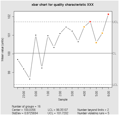
Figure 2: A runaway process
In this case, can we notice that the process is getting out of control before it hits the specification limit? If we can, then do we need to “fix” it?
The answer to the first question is yes, we can notice the trend in the process metric. A number of methods used in Time Series Analysis (TSA) will work here, most common being the correlation analysis. In this case, we check if there is a statistically significant correlation between the timestamp (“Sample” in Figure 2) and the process metric. The standard Pearson’s correlation will do it for most cases, but it will miss nonlinear monotonic correlations, which are just as important. It is better to use Spearman’s correlation test instead.
The answer to the second question is not as obvious. A statistically significant trend in the time series means that there is an external process forcing the metric to change, and the question becomes, do we need to worry about it, or has it always been like that? In other words, we need to determine whether it is “normal” behavior of the process metric.
There is infinitely more to time series analysis than we have outlined in these couple of paragraphs. For more details, please see, e.g., [4].
Trend in an Independent Variable: Time-Series Approach
The easiest way to benchmark a process is to look back and to compare the latest data against the old. If the metric has always been behaving like that, it means that “it is what it is”, the process is experiencing organic growth, and nothing has really changed.
Correlation to time
The idea is to compare the correlation coefficients to time for the baseline and for the recent data. If the correlation has not changed, it is “business as usual”. If it has, then we probably have what Box and Luceno [2] call “attributable cause” behind the change in data behavior.
To do such analysis, it should be possible to perform the T-test on the correlation coefficients for the baseline period and for the latest period of time. The correlation coefficients (Pearson or Spearman), however, do not support such comparison: they are not normally distributed; therefore, the basic assumption of the T-test will not be true. Fortunately, Fisher transform allows us to perform a T- (or Z-) test on the transformed value of the correlation coefficient.
Time-Series Analysis: Regression to time; EWMA; Holt-Winters; ARIMA
Exponentially-weighted moving average, or EWMA (with the Holt-Winters modification to account for the trend and seasonality), predictive filtering is a solid way to benchmark the data: indeed, if we assume that we have a Markov process (the next data point value only depends on the one immediately prior to it), then it does not matter whether the baseline data set is longer than the latest data set, and we can just compare the Holt-Winters predictions. Alternatively, the ARIMA forecasting technique can be utilized.
A definite advantage of the Holt-Winters and ARIMA approach is in that it allows for optimization of the parameters defining how fast the importance of the data point decays as the time goes by. This can be described, in the Holt-Winters case, as a nonlinear-programming (NP) simplex optimization problem.
In-depth discussion of the techniques and their advantages and drawbacks is outside the scope of this paper. For more details, a number of good text can be recommended, most notably [2], [4], and [5]. Each of these methods can produce a prediction of the process metric with some degree of uncertainty. This degree of uncertainty is quantified by the Predictive Interval, or PI, of the forecast.
If the latest data has come outside the Predictive Interval (PI) of what the model said based on the baseline data, then we have a problem. If it is still within the PI, we are ok, and the organic growth is “as expected”.
Selection of the Best Approach to Benchmarking for Time Series Analysis (TSA)
A number of factors play a role in the selection of the best technique, or combination thereof, for SPC through benchmarking. Ultimately, it all depends on the data behavior, and as is usually the case, there is no one-size-fits-all solution.
Whatever the chosen method for selecting the best approach, it all boils down to what is nowadays called machine learning, but really is an automated trial-and-error (T&E) methodology on steroids, since lately massive parallelization has allowed analysts to run multiple models in parallel on the same data sets, selecting the best fitted model when finished, thus reducing greatly the time it takes to compute the forecast.
In addition, the recognition being finally granted lately to the Bayesian methodology, and the development of the “thermodynamics of information” have in the last 15 years made it possible to fit models so as to avoid overfitting and to make likelihood methods, as well as survival modeling, really attractive to the analyst.
Adaptive Alerting (the credit for this section belongs to Dr. Josep Ferrandiz; his blog is here)
Adaptive alerting can be viewed as an application of time-series analysis on steroids: the goal here is to find, at each data point, the new threshold and to verify whether or not the new data point is outside that threshold. In other words, adaptive alerting can be formulated as the problem of detecting statistically significant events as they are happening. In a sense, it means going from an arbitrary physical threshold to a statistically sound percentile (probability) threshold.
Two approaches to Adaptive Alerting
Entropy-based event detection
There are several entropy-based methods of event detection, from traditional Shannon’s entropy-based methods (e.g., the max-likelihood group of methods), to methods based on Second Law of Thermodynamics.
Most notable among the Shannon’s entropy-based methods include max-likelihood methods, among which the most practical are methods based on Akaike Information Criterion (AIC) and Bayesian Information Criterion (BIC). These methods have found wide application in a number of applications, from multidimensional and polynomial regression (keeping the number of variables, or number of degrees of the polynomial, low) to multidimensional clustering.
Methods based on the Second Law of Thermodynamics take advantage of the notion that in a closed system entropy does not decrease. This offers a very efficient way to detect events: entropy going down means the system is not closed anymore, meaning that an external event has changed the system’s behavior.
Residuals-based event detection
Here we compute the best-fitted model (regression or TSA - EWMA and ARIMA) and look at the residuals. An outlier in residuals is an event, and its significance is what determines whether we should alert on it or not.
The standard methodology of hypothesis testing works very well in this case, as it answers the question, “What is the probability that the variable value (or the model residual) will be equal to the one measured if we assume a given distribution of the data?” The given distribution is either the actual distribution of the historical data (or model residuals) or a fitted standard distribution.
Other methods (e.g. [6]) offer innovative ways to use residuals for change-point detection in multidimensional data, where there is a correlation between the two data sets. Time-Series Analysis (TSA) can be interpreted as a special case of multidimensional data and therefore the methods outlined in [6], [8], and a whole host of other publications, can be - and has been - successfully applied to TSA as well.
Stay Tuned for Part 4: Bringing It All Together!
No comments:
Post a Comment