ABSTRACT
Mathematical description of irregular behavior is the holy grail of statistical analysis, akin to a game of croquet that Alice reluctantly played with the Queen of Hearts. (If you have not read or watched Lewis Carroll’s classic, please refer to a brief description of the game here.) A lot of uncertainty and ambiguity, just like in the world of data. In this section, we will discuss one very specific pattern that is critically important in a wide variety of fields, from cardiology to speech recognition, namely seasonality detection.
A Few Words about Seasonality Definitions
First of all, regardless of what Wikipedia says on the page related to Forecasting, seasonality only in some cases has something to do with the four seasons. Or rather, seasonality that is related to the four seasons is only one very special case of seasonality. Wikipedia gives the “right” definition of it on the Seasonality page:
“When there are patterns that repeat over known, fixed periods of time[1] within the data set it is considered to be seasonality,seasonal variation, periodic variation, or periodic fluctuations. This variation can be either regular or semi-regular.”
This is the seasonality that we are going to discuss here.
Seasonality Detection Methods
The most basic method of seasonality detection is to ask the SME (subject-matter expert).
Most SMEs will tell you that their data have a diurnal (a fancy word for “daily”), a weekly, or an annual pattern. But few will tell you that they know what’s going on when the data don’t support their claim.
At this point, we might as well abandon hope to get any useful information from the human SMEs and dive into what the exciting world of machine learning, which in reality is nothing but no-holds-barred advanced statistics, applied, in the seasonality detection use case, to time series.
What is a Time Series?
Time Series is, according to Wikipedia’s article, “a sequence of data points, typically consisting of successive measurements made over a time interval”. NIST is more precise in its definition: “An ordered sequence of values of a variable at equally spaced time intervals”. This definition is the only invariant in time-series analysis. Colloquially, sometimes the word “ordered” is replaced with “time-ordered”.
Seasonality Detection in Time Series
Why?
The most obvious answer to the "why" question is clear from the main use case of Time Series Analysis, - forecasting. Indeed, predicting future behavior of a seasonal time series without accounting for seasonality is akin to driving a small square peg into a big round hole: it fits, but the precision of such model will be poor.
Other use cases include speech recognition, anomaly detection, supply chain management, and stability analysis.
How?
The standard seasonality detection methods, like Fourier analysis, domain expertise, autocorrelation function, etc. work fairly well in most scenarios.
However,
- Domain experts are primarily humans
- Autocorrelation -based seasonality detection involves thresholding, which is only one step better than domain expertise-based seasonality analysis
- Fourier analysis often leads to models that overfit the data
This means that what we are left with is two extremes - too generalized (human) or too specific (Fourier analysis).


An illustration
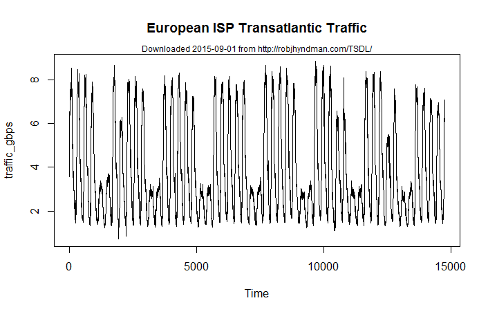
Figure 1: Transatlantic traffic data from a European ISP. Data cover June-July of 2005.
The data are flat enough that we can use this data set to illustrate the concepts we are about to introduce here. To deal with fewer data points, we will go to hourly medians:
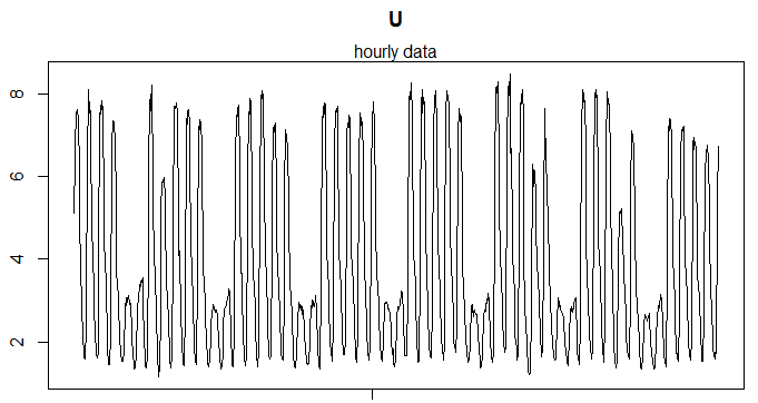
Figure 1a: hourly medians
While it seems fairly obvious visually that there is a daily and a weekly pattern in the data, standard methods will not be very useful. For instance, the AutoCorrelation Function (ACF) returns pretty much the entire spectrum as frequencies:
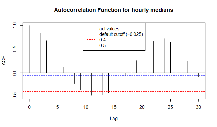
Figure 1b: ACF
Bars whose absolute values are outside the dotted envelope traditionally represent the seasonality.While there is a reason behind the default value of 0.025 (the reason being in Fisherian statistics: if ACF is outside the 5% envelope, we cannot say with 95% confidence that the data are not seasonal); it is clear that with complex seasonal patterns like shown in Figure 1, it is not very meaningful. Expanding the confidence envelope even to 50%, does not contribute much information to our knowledge about these seasonalities.
Looking at Figure 1, we also notice that the upper and the lower parts of the data follow very different patterns: the maxima follow a 2+5 pattern, while the minima follow a daily rhythm with a slight weekly rhythm. It is understandable if we recall that these data correspond to traffic through a large Internet Service Provider (ISP) in a very busy time of a year - June/July.
Let’s follow through with the ROC idea and see where it brings us.


Figure 3: ROC time Series plot.
Points following ROC change of sign are marked as red dots; all others are blank dots.


Figure 4. Hour-to-Hour variability in traffic
In Figure 4(b), the points after which the sign of the first derivative changed from positive to negative correspond to the local maxima of the hourly median time series. They are marked as blue filled dots. Points where second derivative changes sign are inflection points. These are marked as boxes.
Let us look at the distribution of the time intervals between the sign-change points.
We see that the density plot, too, has multiple local maxima.
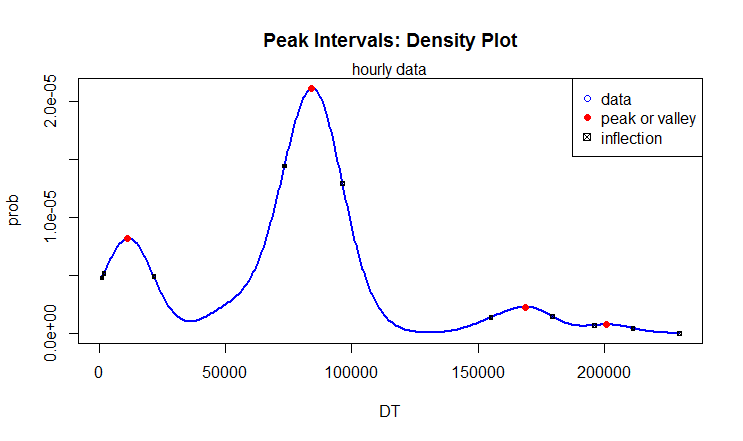
(a): Distribution of intervals between peaks (seconds)
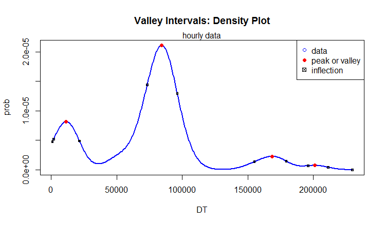
(b): Distribution of intervals between valleys (seconds)
Figure 7: Density of time intervals between local maxima and minima of hourly traffic medians.
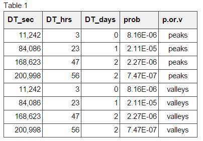
We see from Figure 7 (a & b) that peaks and valleys of the hourly traffic medians follow the same pattern. Table 1 verifies this. The peaks are observed at 3, 23, 47, and 56 hours, and so are the valleys.
Their complex interactions and interferences, not unlike the Wave Pendulum, produces the pattern we saw in Figure 1.
Conclusion
We have demonstrated a reliable method of detecting complex seasonal patterns in time series data. This method does not require Fourier decomposition, regression fitting, Neural Networks, or any other overkill techniques. All that is needed is high-school Calculus, Probability and Statistics, fundamental understanding of Clustering, and a little common sense.

