Predictive SPC. Part 5
Statistical Process Control (SPC) is a well described framework used to identify weak points in any process and predict the probability of failure in it. The distribution parameters of process metrics have been translated into process capability, which evolved in the 1990s into the Six Sigma methodology in a number of incarnations. However, all techniques derived for SPC have two important weaknesses: they assume that the process metric is in a steady state and they assume that the process metric is normally distributed, or can be converted to a normal distribution. The concepts and ideas outlined here make it possible to overcome these two shortcomings. This method has been developed and validated in collaboration with Josep Ferrandiz.
This is the concluding post in the series on Predictive SPC.
Definitions are here.
In Part 1, we covered the Axioms and Assumptions (A&As) of SPC, explained why they are wrong, but useful. In Part 2, we talked about the key concepts and ideas of SPC, and Part 3 had a discussion of how the key SPC concepts and ideas will change if we consider non-stationary processes. Finally, in Part 4, we brought it all together, and now we are moving on to an illustration of the methodology.
Method Illustration
Examples that we are using for illustration are taken from the world of Client-Server applications in IT. The business objective in IT operations is, among many, to always stay ahead of the business curve, so that when the new business opportunities propel the company to new levels, there is enough hardware to sustain it. One of the ways to do it is to reduce the amount of resource needed to sustain a given business rate. In IT, the KPM can be traffic (Concurrency = number of concurrent queries in the system at any time), CPU load, memory utilization, data flow rate, latency, etc. The BMI can be transaction rate, revenue, all kinds of confidence indices, etc.
Figure 4 shows the values of the chosen KPM as predicted by the same model based on the data observed in the Baseline and data observed in the new data set. Figure 4 shows that the traffic became higher in the new time frame than it was during the Baseline time segment: the nature of the data changed. The second-order (quadratic) component in the relationship between the KPM and the business metric is now statistically significant.
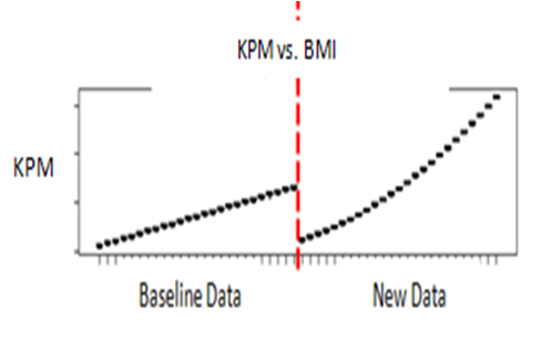
Figure 4: Illustration of Process Degradation:
predictions from the model built on the baseline data are to the left of the dividing vertical line; predictions based on the recent data are to the right.
In this this particular application, the same model, applied to baseline and new data, predicted vastly different KPM values: new data gave much higher numbers than baseline. We find that the W varies from +0.5 at low values of the business metric to +5.3 at high BMI. Conclusion: this application has recently degraded.
Positive values of the W score indicate process degradation.
On the other hand, Figure 5 shows another case, where the W went from -0.2 to -7.4
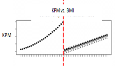
Figure 5: Illustration of Process Improvement:
predictions from the model built on the baseline data are to the left of the dividing vertical line; predictions based on the recent data are to the right.
In Figure 5, the same model applied to new data shows lower values of KPM than when it was applied to the baseline data. The negative value of the W indicates process improvement, and in this case we find W = -0.2 at lower BMI values and W = -7.4 in the high-BMI zone.
Usage
Figures 4 and 5 present illustrations of the use of the method when the system degraded (Figure 4) and the system improved (Figure 5). Figure 6 presents the algorithm that we implemented for Predictive SPC.
For reasons of information sensitivity, all the data in this post have been generated to replicate patterns similar to what one usually sees in the real IT production environment.

Figure 6: Predictive SPC core algorithm
The strength of the core algorithm in Figure 6 is in its applicability to multiple entities and its metric-ignorance: it can provide a single-number measure of enterprise-wide performance quality, regardless of the metrics used for a particular facet of the performance.
The output can be visualized using Heat Maps, Dashboards, and other techniques. Standard off the shelf data visualization tools, such as Tableau, SAS, R visualization packages (ggplot2 and / or lattice), as well as specialized tools, can be used to provide high-quality graphics.
Enterprise-level applicability
The main requirements for enterprise-level applicability of the method we are describing, namely scalability and ease of interpretation, are met by using parallel processing and visualization. HeatMaps offer a great way to visualize many metrics for multiple entities at once, but that is outside the scope of this post. The W as a measure of process consistency offers a way to identify the worst and the best applications (high and low outliers, respectively), “Top 10” units, etc.
Conclusions
This is the final post in the series describing a novel, robust, reliable, scalable, self-consistent, and easy-to-interpret methodology for measuring process quality in a non-stationary system.
This methodology can be extended to stationary processes and therefore is inclusive of the current state of the art. Needless to say, the KPM, BMI, and other terms were used throughout the paper for the sole purpose of illustration.
A way to establish a quantile regression model in cases where the model structure is unknown has been outlined in general terms here. In implementation of polynomial models, it is important to have a conditional model substitution (see here). Linear or exponential models may be better predictors in such cases, even if their correlation coefficient is not as good as for polynomial.
This methodology can be used with any system where a predictive model can be applied to the baseline and recent data. There is no need to normalize the data by applying the Box-Cox and other transformations: the methods we are using are entirely non-parametric.
This Predictive SPC methodology has been successfully implemented in an Enterprise-level tool for IT in an environment where stationarity is not to be expected. The tool implementing this methodology can be used to quickly (within two weeks) highlight the problems with new production releases and help the engineers identify and fix the problems whose identification alone would otherwise have taken several months.
And that concludes the series on Predictive SPC
References
[1] Ricci, V. (2005). Fitting Distributions with R. http://cran.r-project.org/doc/contrib/Ricci-distributions-en.pdf Downloaded 06/02/2010.
[2] Box, G.E.P, Luceno, A. (Eds.) (1997) Statistical Control by Monitoring and Feedback Adjustment; Wiley Series in Probability and Statistics; Copyright 1997, John Wiley and Sons, Inc.; ISBN 0-471-19046-2
[3] Josep Ferrandiz, Alex Gilgur. (2012) Level of Service Based Capacity Planning. – published at the 38th International Computer Measurement Group (CMG12) Conference, December 2012, Las Vegas, NV.
[4] Chapman, C. (2003) Analysis of Time Series. An Introduction (6th ed.) Chapman and Hall, 2003.
[5] Shumway, R.H., Stoffer, D.S. (2006) Time Series Analysis and Its Applications with R examples, 2nd.ed. Springer Texts in Statistics; Copyright 2006. ISBN 0-387-29317-5.
[6] Josep Ferrandiz, Alex Gilgur. (2012) A Note on Knee Detection. – published at the 38th International Computer Measurement Group (CMG12) Conference, December 2012, Las Vegas, NV.
[7] Alexander Gilgur, Michael Perka (2006). A Priori Evaluation of Data and Selection of Forecasting Model – published at the 32nd International Computer Measurement Group (CMG06) Conference, December 2012, Reno, NV.
[8] Alex Gilgur,Josep Ferrandiz, Matthew Beason. (2012) Time-Series Analysis: Forecasting + Regression: And or Or? – published at the 38th International Computer Measurement Group (CMG12) Conference, December 2012, Las Vegas, NV.
[9] Alex Gilgur. Little’s Law assumptions: “But I still wanna use it!” The Goldilocks solution to sizing the system for non-steady-state dynamics. CMG MeasureIT journal, Iss. 13.6, June, 2013. http://www.cmg.org/measureit/issues/mit100/m_100_6.pdf
No comments:
Post a Comment